

Chapter Resources
- A note on simulation software
- Thinking like a population geneticist
- Genotype frequencies
- Genetic drift and effective population size
- Population structure and gene flow
- Mutation
- Fundamentals of natural selection
- Further models of natural selection
- Molecular evolution
- Quantitative trait variation and evolution
- The Mendelian basis of quantitative trait variation
- Historical and synthetic topics
- Appendix
A note on simulation software
Be sure to read any installation instructions provided with the software linked below. The software referenced here has been designed to install easily and to be user-friendly. Nonetheless, paying attention to the instructions will help insure that any applications install and then run as intended by their authors.
The program PopGene.S2 is written in Microsoft visual basic. The program requires a code library called ".NET framework 2.0 in order to run. Most Windows computers will require an update to .NET framework 2.0. This update only needs to be installed once. The .NET framework 2.0 update can be found by opening the web page http://www.microsoft.com/downloads/ and then searching for ".NET framework 2.0"
Chapter 1
There is no additional content for this chapter.
Chapter 2
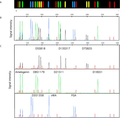
[Figure caption] An electropherogram of a ten locus DNA fragment genotype from a capillary DNA sequencer. This is a full color version of Figure 2.8 in the text.
Interact Boxes 2.1 - 2.4
PopGene.S2 [http://www9.georgetown.edu/faculty/hamiltm1/Text_book.html] is a simulation application that carries out a variety of informative population genetics simulations. PopGene.S2 requires a computer running Microsoft Windows 95 or later.
Interact Box 2.5
Populus (http://www.cbs.umn.edu/populus/) is an application that carries out a wide range of genetic and ecological simulations. It is available in an older DOS version (3.42) that can run on most computers with current versions of the Windows operating system. It is also available in a Java version for Windows, Macintosh OSX, and Linux. Go to the Download page to obtain the version that runs on the computer you will use. Consider obtaining both version 3.42 for DOS as well as the Java version if you are using a Windows computer. The older DOS version has a more complete version of the parent-offspring regression simulation compared to the Java version.
Download a simple simulation of recombination with natural selection constructed in Microsoft Excel.
Interact Box 2.6
Genepop on the Web (http://genepop.curtin.edu.au)
Download a microsatellite genotype data set containing three loci from Chesapeake Bay striped bass (Morone saxatilis) in Genepop format to explore how genotype disequilibrium tests work.
Steps:
- Use a web browser to reach the main Genepop page.
- Then select Option 2 for genotypic disequilibrium tests.
- On the Option 2 page, select a radio button under the heading Diploid Data: Genotypic disequilibrium. Suboption 1. (Test for each pair of loci in each population) will carry out a statistical test that genotype counts are pairs of loci are randomly distributed, while Suboption 2 (Only Create genotypic contingency tables) will just show the contingency tables. I suggest trying suboption 2 first and then suboption 1 later. Leave the Markov chain parameters as the default values and check the boxes to set where the output will be delivered.
- Next, open the data set in a text editor program and copy the entire contents of the file.
- Then return to the Genepop web page and paste the data set into the dialog at the bottom of the page.
- Select the 2-Digit Alleles (00-99) radio button. Once all of the options are selected, click on the Submit data button.
The contingency table shown in the book will be the 6th table down in the output from Genepop.
Chapter 3
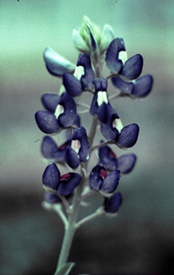
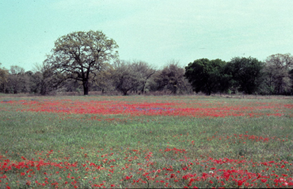
[Figure caption] The Texas bluebonnet (Lupinus texensis) is a plant often found in continuous populations of hundreds or thousands of individuals that cover large areas. In the photo above the blue flowers in the center of the picture are L. texensis (the red flowers are Phlox drummondii). Despite the overall large numbers of individuals, the genetic neighborhood size of L. texensis is only about 95 individuals since gamete and seed dispersal shows strong isolation by distance. Photos by Dr. Barbara Schaal, used with permission.
Interact Box 3.1
Populus http://www.cbs.umn.edu/populus/
Interact Box 3.2
PopGene.S2: http://www9.georgetown.edu/faculty/hamiltm1/Text_book.html
Interact Box 3.3
Populus http://www.cbs.umn.edu/populus/
Interact Box 3.4
Construct your own coalescent trees using this Microsoft Excel spreadsheet to simulate waiting times: Download basic coalescent spreadsheet (Version 2)
NOTE: Microsoft Excel 2008 (v12.2.7 tested) for the Macintosh has a known bug that causes spread sheets with the vlookup function or with very large data sets to execute very slowly. Since this spread sheet utilizes the vlookup function and contains a very large set of numerical values, it may take several minutes to open or to update when saved. This is not a problem with the spread sheet itself. The recommended work around is to use another version of Excel. These files were tested with Excel 2004 (v11.6.2 tested) for the Macintosh and found to open and recalculate normally.
Interact Box 3.5
Simulate gene genealogies under the coalescent model using this web page: http://www.coalescent.dk/ Click on WrightFisher animator link and then the WrightFisher link.
Interact Box 3.6
Simulate gene genealogies in a population growing exponentially over time using this web page: http://www.coalescent.dk/ Click on the Hudson animator link and then the Exponential growth link. Note that there is a help page link on the Hudson animator page. An alternative coalescent simulator for exponentially growing populations is: TreeToy http://www.xmission.com/~wooding/TreeToy/ Treetoy is used in Interact Box 8.3
Chapter 4
Interact Box 4.1
Estimate the average exclusion probabilities in paternity analysis for loci with 6 and 12 alleles using this Microsoft Excel spreadsheet: Download average exclusion probabilities spreadsheet
Interact Box 4.2
PopGene.S2 http://www9.georgetown.edu/faculty/hamiltm1/Text_book.html Click on the Gene Flow and Subdivision menu and then Wahlund effect. For a web-based simulation of the Wahlund effect go to: http://darwin.eeb.uconn.edu/simulations/wahlund.html
Interact Boxes 4.3 4.5
PopGene.S2 http://www9.georgetown.edu/faculty/hamiltm1/Text_book.html
Interact Box 4.6
Simulate gene genealogies under the combined processes of coalescece and gene flow using this web page: http://www.coalescent.dk/ Click on the Hudson animator link and then the Migration link.
Chapter 5
Interact Boxes 5.1 and 5.2
PopGene.S2 http://www9.georgetown.edu/faculty/hamiltm1/Text_book.html
Interact Box 5.3
Compare estimates of population structure under the infinite alleles model and the stepwise mutation model using this Microsoft Excel spreadsheet: Download FST and RST comparison spreadsheet
Interact Box 5.4
Simulate irreversible and bi-directional mutation: PopGene.S2 http://www9.georgetown.edu/faculty/hamiltm1/Text_book.html
Interact Box 5.5
Construct you own genealogical trees under the combined processes of coalescence and mutation using this Microsoft Excel spreadsheet: Download coalescence and mutation spreadsheet (Version 2)
NOTE: Microsoft Excel 2008 (v12.2.7 tested) for the Macintosh has a known bug that causes spread sheets with the vlookup function or with very large data sets to execute very slowly. Since this spread sheet utilizes the vlookup function and contains a very large set of numerical values, it may take several minutes to open or to update when saved. This is not a problem with the spread sheet itself. The recommended work around is to use another version of Excel. These files were tested with Excel 2004 (v11.6.2 tested) for the Macintosh and found to open and recalculate normally.
Chapter 6
Interact Box 6.1
Populus http://www.cbs.umn.edu/populus/
Chapter 7
Interact Boxes 7.1 7.3
Populus http://www.cbs.umn.edu/populus/
Interact Boxes 7.4 and 7.5
PopGene.S2 http://www9.georgetown.edu/faculty/hamiltm1/Text_book.html
Interact Box 7.6
Simulate gene genealogies with directional selection using this web page: http://www.coalescent.dk/ Click on Hudson animator link and then the Selection link. Note that there is a help page link on the Hudson animator page.
Chapter 8
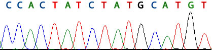
[Figure caption] A color electropherogram of DNA sequence from a capillary DNA sequencer. This is a full color version of Figure 8.6 in the text.
Interact Box 8.1
Populus http://www.cbs.umn.edu/populus/
PopGene.S2 http://www9.georgetown.edu/faculty/hamiltm1/Text_book.html
Interact Box 8.2
PopGene.S2 http://www9.georgetown.edu/faculty/hamiltm1/Text_book.html
Download a data set of 30 DNA sequences from African sable antelope in FASTA format to explore nucleotide diversity and segregating sites.
Steps:
- Use a web browser to reach the main Genbank page http://www.ncbi.nlm.nih.gov/
- Search Popset (use the popout menu) for accession 13958252 by entering this number in the search field at the top of the page and clicking the Go button.
- On the search results page, click on the Pitra C link.
- The DNA sequence data will be shown. Scroll down the page to view the data.
- Change the display format of the DNA sequences.
- At the top left-hand corner of the page showing the DNA data there is a popout menu with the heading Display. Choose the FASTA option in this menu. The page will refresh and the data will be shown in FASTA format.
- Next, save the DNA sequences to a file that can be read by PopGene.S2.
- To the right of the Display menu is another popout menu titled Send to that is used to export the data. Click on that menu and select the File option. A file will download to your computer (usually named sequences.seq).
- Find the downloaded file on your computer and rename it to end with .fas. An example file name would be antelope_mtdna.fas.
Launch PopGene.S 2 and follow the instructions in Interact Box 8.2.
If you had trouble obtaining the data from Genbank, download the file directly here.
Problem Box 8.2
The FASTA sequence files are: mayotte_runt.fas and europe_runt.fas Multiple sequence alignment files in the MEGA format are: mayotte_runt_aligned.meg and europe_runtt_aligned.meg The MEGA files can be opened in both MEGA and DNAsp to compute Tajima's D.
Interact Box 8.3
Simulate genealogies with neutral mutations in populations that are growing exponentially over time. This simulation can be used to understand the relationship between population growth and the haplotype frequency spectrum and the mismatch distribution: TreeToy http://www.xmission.com/~wooding/TreeToy/
Chapter 9
Interact Box 9.1
Populus http://www.cbs.umn.edu/populus/
1. Launch Populus and from the Models menu choose Quantitative-Genetic models and then Heritability. Start with the default values in the dialog box. Once you press the view button, the simulation begins. Changing the model parameter values will change the simulation results. There are two radio buttons to select the theoretical or Monte Carlo versions of the simulation. In the Monte Carlo version of the model pressing the space bar will take a new random sample of data (try this now). Note that the default values are p = 0.3 and Ne = 250.
Question: For the theoretical model what do the distributions outlined in green and blue represent? For the Monte Carlo model what do the circles and the green and blue histograms represent?
2. View the theoretical model. Increase and decrease the value of VE.
Question: What happens to the heritability? Biologically what is VE? Why does it impact the heritability?
3. View the theoretical model. Increase and decrease the allele frequency in the population (p). Try p = 0.5 and p = 0.05.
Question: What happens to the heritability? Why does the allele frequency impact the heritability?
4. View the Monte Carlo model and press the space bar a few times. Notice that pressing the space bar with the theoretical model does nothing. Also try setting the value of Ne to 250 and 30 while pressing the space bar.
Question: What is the fundamental difference between the theoretical and Monte Carlo models?
5. View the Monte Carlo model with p = 0.5 and VE = 0.
Question: Why are there clumps of data points? How many clumps of data points are there and why?
6. In the model dialog G1, G2 and G3 represent the genotypic values for each of the three genotypes AA, Aa and aa. Genotypic values are the phenotype that an individual of a given genotype will possess if there is no environmental impact on phenotype. As an example, imagine the locus in the model causes the phenotype of butterfly spots and that an AA homozygote has 15 spots, an Aa heterozygote has 10 spots, and an aa homozygote has 5 spots. View the Theoretical graph. Set G1 = 5, G2 = 10 and G3 = 15. Set VE = 0.1.
Question: What is h2?
Now set G1 = 5, G2 = 11 and G3 = 15. Set VE = 0.1.
Question: What is h2?
Finally set G1 = 5, G2 = 13 and G3 = 15. Set VE = 0.1.
Question: What is h2?
[Note: The version of Populus available at the time of this writing had bugs in the parentoffspring regression simulation. For certain genotypic values that represent dominance (e.g. G1 = 5, G2 = 15 and G3 = 15) the heritability given by the program was not correct although the slope of the line appeared to be as expected.]
Why does the heritability decline as G2 increases in value? Think of the difference between the effect of a genotype on phenotype on the one hand and what progeny inherit from their parents on the other hand.
7. Switch to the Monte Carlo model. Set VE = 0. Repeat the progression in the value of G2 as in step 6 above. Explain why heritability declines in value by referring to the patterns of circles and the slope of the regression line. Why do the circles cluster as the value of G2 approaches the value of G3?
Summary Questions
(Answer these by referring to patterns seen in the simulations):
Why is the narrow-sense heritability used to predict the change in the mean of a quantitative phenotype caused by natural selection?
What does natural selection do to the frequency of alleles in the next generation?
Why is natural selection not as effective in changing the mean of a phenotype that has a lot of dominance genetic variation (VD)?
Interact Box 9.2
Computing the predicted response to selection on multiple traits requires matrix algebra. Those familiar with matrix algebra may be able to determine the inverse of a small matrix or dot product of two matrices. For those not familiar with matrix algebra or not wanting to carry out the computations by hand, the Matlab code below will compute Δz¯ (or delta z-bar) for two phenotypes given G and P matrices and a vector s of selection differentials.
function delta_z_bar
% function to compute the change in mean phenotype (delta_z_bar) from:
% P - the phenotypic variance-covariance matrix
% G - the genotypic variance-covariance matrix
% s - the column vector of selection differentials
P = [1, 0;
0, 1.5];
G = [0.5, 0;
0, 0.5];
s = [0.5;
0.5];
% first, get the inverse of P
Pinv = inv(P);
% then solve for delta_z_bar
delta_z_bar = G*Pinv*s
Interact Boxes 9.3 - 9.4
PopGene.S2 http://www9.georgetown.edu/faculty/hamiltm1/Text_book.html
Interact Box 9.5
PopGene.S2 http://www9.georgetown.edu/faculty/hamiltm1/Text_book.html
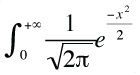
When truncation selection is applied, determining the selection differential requires determining the mean of the parental phenotypic distribution above the truncation point. This can be done using the partial moments of a normal distribution. In general, the partial moment of a normal distribution is integral[0, +infinity] ([1/sqrt(2π)] * e-x2/2). or
With a normal distribution that has a mean of zero, a variance of sigma2 and a truncation point of t, the mean of the portion of the distribution between t and +infinity is
[sigma/sqrt(2π)] * e-t2/(2*sigma2) . or
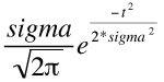
In the case where the trunction point is at the 50th percentile of the distribution, the trunction point is the mean of the distribution and t = 0. With sigma = 1 the mean of the distribution above the trunction point is 1/[square root(2π)] = 0.39894.
Chapter 10
Interact Box 10.1
Graph the average effect, breeding value and dominance deviation for the three genotypes at one locus using this Microsoft Excel spreadsheet: Download average effect, breeding value, and dominance deviation spreadsheet
Interact Box 10.2
Graph the components of the genotypic variance (VG, VA & VD) using this Microsoft Excel spreadsheet: Download components of genotypic variance spreadsheet
Chapter 11
There is no additional content for this chapter.
Appendix
Interact box A.1
Central limit theorem simulation: http://www.ruf.rice.edu/~lane/stat_sim/sampling_dist/ (see another central limit theorem simulator based on dice: http://www.stat.sc.edu/~west/javahtml/CLT.html)